November 2008 | Industrial Automation and Mechatronics

What are Level Controllers?

Level controllers monitor, regulate, and control liquid or solid levels in a process. There are three basic types of control functions that level controllers can use. Limit control works by interrupting power through a load circuit when the level exceeds or falls below the limit set point. A limit controller can protect equipment and people when it is correctly installed with its own power supply, power lines, switch and sensor. Advanced or non-linear control includes dead-time compensation, lead/lag, adaptive gain, neural networks, and fuzzy logic. Level controllers can be used for either liquid or powder or other dry material applications.

Linear level controllers can take many different styles. Feedforward control offers direct control or compensation from the reference signal. It may be open loop or in conjunction with PID control. Proportional, integral, and derivative (PID) control is an intelligent I/O module or program instruction, which provides automatic closed-loop operation of process control loops. Proportional plus integral (PI) control has the error signal integrated and is used for eliminating steady state or offset errors. It may also be called automatic reset/bias/offset control.

Proportional plus derivative (PD) control has the error signal differentiated to get the rate of change. This type of control is used to increase controller speed of response, but can be noisy and make the system less stable. In proportional (P) control, the control signal is proportional to the error between the reference and feedback signals.

Level controllers differ in terms of specifications, user interface, and features. Specifications include the number of inputs, control outputs and control feedback loops. Control loops may be linked to improve control performance and/or stability. The control output is usually analog current, voltage or a switched output. These controllers can have discrete or TTL I/O as well and can handle high power switching needs. The user interface for level controllers may be analog, digital or computer controlled. Displays for level controllers can be analog meters, digital numerical readouts, or video display terminals. Another possible type of display is a strip chart or circle chart. When connecting to a computer host, level controllers can use the standard serial, parallel or SCSI interfaces or can be networkable via Ethernet, CANBus or a number of other network protocols. Features that are sometimes optional for level controllers include sensor excitation current or voltage, built-in alarms or indicators and washdown or waterproof ratings. Other features can include programmable setpoints, autotune or self-tuning functions and signal computation functions or filters.

Level sensors are used to detect liquid or powder levels, or interfaces between liquids. These level measurements can be either continuous or point values represented with various output options. Continuous level sensors are devices that measure level within a specified range and give output of a continuous reading of level. Point level sensors devices mark a specific level, generally used as high alarm or switch.

Multiple point sensors can be integrated together to give a stepped version of continuous level. These level sensors can be either plain sensors with some sort of electrical output or else can be more sophisticated instruments that have displays and sometimes computer output options. The measuring range is probably the most important specification to examine when choosing a level sensor. Field adjustability is a nice feature to have for tuning the instrument after installation.

Depending on the needs of the application, level sensing devices can be mounted a few different ways. These sensors can be mounted on the top, bottom or side of the container holding the substance to be measured. Among the technologies for measuring level are air bubbler technology, capacitive or RF admittance, differential pressure, electrical conductivity or resistivity, mechanical or magnetic floats, optical units, pressure membrane, radar or microwave, radio frequency, rotation paddle, ultrasonic or sonic and vibration or tuning fork technology. Analog outputs level sensors can be current or voltage signals. Also possible is a pulse or frequency. Another option is to have an alarm output or a change in state of switches. Computer signal outputs that are possible are usually serial or parallel. Level sensors can have displays that are analog, digital or video displays. Control for the devices can be analog with switches, dials and potentiometers; digital with menus, keypads and buttons; or controlled by a computer.

What is Statistical Process Control SPC?

Statistical process control (SPC) is a method for achieving quality control in manufacturing processes. It is a set of methods using statistical tools such as mean, variance and others, to detect whether the process observed is under control.

Statistical process control was pioneered by Walter A. Shewhart and taken up by W. Edwards Deming with significant effect by the Americans during World War II to improve industrial production. Deming was also instrumental in introducing SPC methods to Japanese industry after that war. Dr. Shewhart created the basis for the control chart and the concept of a state of statistical control by carefully designed experiments. While Dr. Shewhart drew from pure mathematical statistical theories, he understood data from physical processes never produce a "normal distribution curve" (a Gaussian distribution, also commonly referred to as a "bell curve"). He discovered that observed variation in manufacturing data did not always behave the same way as data in nature (Brownian motion of particles).
Dr. Shewhart concluded that while every process displays variation, some processes display controlled variation that is natural to the process, while others display uncontrolled variation that is not present in the process causal system at all times.

Classical Quality control was achieved by observing important properties of the finished product and accept/reject the finished product. As opposed to this technique, statistical process control uses statistical tools to observe the performance of the production line to predict significant deviations that may result in rejected products.

The underlying assumption in the SPC method is that any production process will produce products whose properties vary slightly from their designed values, even when the production line is running normally, and these variances can be analyzed statistically to control the process. For example, a breakfast cereal packaging line may be designed to fill each cereal box with 500 grams of product, but some boxes will have slightly more than 500 grams, and some will have slightly less, producing a distribution of net weights. If the production process itself changes (for example, the machines doing the manufacture begin to wear) this distribution can shift or spread out. For example, as its cams and pulleys wear out, the cereal filling machine may start putting more cereal into each box than it was designed to. If this change is allowed to continue unchecked, product may be produced that fall outside the tolerances of the manufacturer or consumer, causing product to be rejected.

By using statistical tools, the operator of the production line can discover that a significant change has been made to the production line, by wear and tear or other means, and correct the problem - or even stop production - before producing product outside specifications. An example of such a statistical tool would be the Shewhart control chart, and the operator in the aforementioned example plotting the net weight in the Shewhart chart.

What is Industrial Automation?

Automation (ancient Greek: = self dictated), roboticization or industrial automation or numerical control is the use of control systems such as computers to control industrial machinery and processes, replacing human operators. In the scope of industrialization, it is a step beyond mechanization. Whereas mechanization provided human operators with machinery to assist them with the physical requirements of work, automation greatly reduces the need for human sensory and mental requirements as well.

Currently, for manufacturing companies, the purpose of automation has shifted from increasing productivity and reducing costs, to broader issues, such as increasing quality and flexibility in the manufacturing process.

The old focus on using automation simply to increase productivity and reduce costs was seen to be short-sighted, because it is also necessary to provide a skilled workforce who can make repairs and manage the machinery.

Moreover, the initial costs of automation were high and often could not be recovered by the time entirely new manufacturing processes replaced the old. (Japan's "robot junkyards" were once world famous in the manufacturing industry.)

Automation is now often applied primarily to increase quality in the manufacturing process, where automation can increase quality substantially. For example, automobile and truck pistons used to be installed into engines manually. This is rapidly being transitioned to automated machine installation, because the error rate for manual installment was around 1-1.5%, but has been reduced to 0.00001% with automation. Hazardous operations, such as oil refining, the manufacturing of industrial chemicals, and all forms of metal working, were always early contenders for automation.

Another major shift in automation is the increased emphasis on flexibility and convertibility in the manufacturing process. Manufacturers are increasingly demanding the ability to easily switch from manufacturing Product A to manufacturing Product B without having to completely rebuild the production lines.

What is an LVDT and other information...

What is an LVDT?

The letters LVDT are an acronym for Linear Variable Differential Transformer, a common type of electromechanical transducer that can convert the rectilinear motion of an object to which it is coupled mechanically into a corresponding electrical signal. LVDT linear position sensors are readily available that can measure movements as small as a few millionths of an inch up to several inches, but are also capable of measuring positions up to ±20 inches (±0.5 m).

Structure of a typical LVDT

The figure shows the components of a typical LVDT. The transformer's internal structure consists of a primary winding centered between a pair of identically wound secondary windings, symmetrically spaced about the primary. The coils are wound on a one-piece hollow form of thermally stable glass reinforced polymer, encapsulated against moisture, wrapped in a high permeability magnetic shield, and then secured in a cylindrical stainless steel housing. This coil assembly is usually the stationary element of the position sensor.

The moving element of an LVDT is a separate tubular armature of magnetically permeable material called the core, which is free to move axially within the coil's hollow bore, and mechanically coupled to the object whose position is being measured. This bore is typically large enough to provide substantial radial clearance between the core and bore, with no physical contact between it and the coil.

In operation, the LVDT's primary winding is energized by alternating current of appropriate amplitude and frequency, known as the primary excitation. The LVDT's electrical output signal is the differential AC voltage between the two secondary windings, which varies with the axial position of the core within the LVDT coil. Usually this AC output voltage is converted by suitable electronic circuitry to high level DC voltage or current that is more convenient to use.

Why use an LVDT?

LVDTs have certain significant features and benefits, most of which derive from its fundamental physical principles of operation or from the materials and techniques used in its construction.

Friction-Free Operation

One of the most important features of an LVDT is its friction-free operation. In normal use, there is no mechanical contact between the LVDT's core and coil assembly, so there is no rubbing, dragging or other source of friction. This feature is particularly useful in materials testing, vibration displacement measurements, and high resolution dimensional gaging systems.

Infinite Resolution

Since an LVDT operates on electromagnetic coupling principles in a friction-free structure, it can measure infinitesimally small changes in core position. This infinite resolution capability is limited only by the noise in an LVDT signal conditioner and the output display's resolution. These same factors also give an LVDT its outstanding repeatability.

Unlimited Mechanical Life

Because there is normally no contact between the LVDT's core and coil structure, no parts can rub together or wear out. This means that an LVDT features unlimited mechanical life. This factor is especially important in high reliability applications such as aircraft, satellites and space vehicles, and nuclear installations. It is also highly desirable in many industrial process control and factory automation systems.

Overtravel Damage Resistant

The internal bore of most LVDTs is open at both ends. In the event of unanticipated overtravel, the core is able to pass completely through the sensor coil assembly without causing damage. This invulnerability to position input overload makes an LVDT the ideal sensor for applications like extensometers that are attached to tensile test samples in destructive materials testing apparatus.

Single Axis Sensitivity

An LVDT responds to motion of the core along the coil's axis, but is generally insensitive to cross-axis motion of the core or to its radial position. Thus, an LVDT can usually function without adverse effect in applications involving misaligned or floating moving members, and in cases where the core doesn't travel in a precisely straight line.

Separable Coil And Core

Because the only interaction between an LVDT's core and coil is magnetic coupling, the coil assembly can be isolated from the core by inserting a non-magnetic tube between the core and the bore. By doing so, a pressurized fluid can be contained within the tube, in which the core is free to move, while the coil assembly is unpressurized. This feature is often utilized in LVDTs used for spool position feedback in hydraulic proportional and/or servo valves.

Environmentally Robust

The materials and construction techniques used in assembling an LVDT result in a rugged, durable sensor that is robust to a variety of environmental conditions. Bonding of the windings is followed by epoxy encapsulation into the case, resulting in superior moisture and humidity resistance, as well as the capability to take substantial shock loads and high vibration levels in all axes. And the internal high-permeability magnetic shield minimizes the effects of external AC fields.

Both the case and core are made of corrosion resistant metals, with the case also acting as a supplemental magnetic shield. And for those applications where the sensor must withstand exposure to flammable or corrosive vapors and liquids, or operate in pressurized fluid, the case and coil assembly can be hermetically sealed using a variety of welding processes.

Ordinary LVDTs can operate over a very wide temperature range, but, if required, they can be produced to operate down to cryogenic temperatures, or, using special materials, operate at the elevated temperatures and radiation levels found in many nuclear reactors.

Null Point Repeatability

The location of an LVDT's intrinsic null point is extremely stable and repeatable, even over its very wide operating temperature range. This makes an LVDT perform well as a null position sensor in closed-loop control systems and high-performance servo balance instruments.

Fast Dynamic Response

The absence of friction during ordinary operation permits an LVDT to respond very fast to changes in core position. The dynamic response of an LVDT sensor itself is limited only by the inertial effects of the core's slight mass. More often, the response of an LVDT sensing system is determined by characteristics of the signal conditioner.

Absolute Output

An LVDT is an absolute output device, as opposed to an incremental output device. This means that in the event of loss of power, the position data being sent from the LVDT will not be lost. When the measuring system is restarted, the LVDT's output value will be the same as it was before the power failure occurred.

How does an LVDT work?

This figure illustrates what happens when the LVDT's core is in different axial positions. The LVDT's primary winding, P, is energized by a constant amplitude AC source. The magnetic flux thus developed is coupled by the core to the adjacent secondary windings, S1 and S2 . If the core is located midway between S1 and S2 , equal flux is coupled to each secondary so the voltages, E1 and E2 , induced in windings S1 and S2 respectively, are equal. At this reference midway core position, known as the null point, the differential voltage output, (E1 - E2 ), is essentially zero.

LVDT Core Position Diagram

If the core is moved closer to S1 than to S2 , more flux is coupled to S1 and less to S2 , so the induced voltage E1 is increased while E2 is decreased, resulting in the differential voltage (E1 - E2). Conversely, if the core is moved closer to S2 , more flux is coupled to S2 and less to S1 , so E2 is increased as E1 is decreased, resulting in the differential voltage (E2 - E1 ).

The top graph shows how the magnitude of the differential output voltage, EOUT, varies with core position. The value of EOUT at maximum core displacement from null depends upon the amplitude of the primary excitation voltage and the sensitivity factor of the particular LVDT, but is typically several volts RMS. The phase angle of this AC output voltage, EOUT, referenced to the primary excitation voltage, stays constant until the center of the core passes the null point, where the phase angle changes abruptly by 180 degrees, as shown in the middle graph.

This 180 degree phase shift can be used to determine the direction of the core from the null point by means of appropriate circuitry. This is shown in the bottom graph, where the polarity of the output signal represents the core's positional relationship to the null point. The figure shows also that the output of an LVDT is very linear over its specified range of core motion, but that the sensor can be used over an extended range with some reduction in output linearity. The output characteristics of an LVDT vary with different positions of the core. Full range output is a large signal, typically a volt or more, and often requires no amplification. Note that an LVDT continues to operate beyond 100% of full range, but with degraded linearity.

From Macro Sensors website

What are Temperature Transmitters?

Temperature measurement using modern scientific thermometers and temperature scales goes back at least as far as the early 18th century, when Gabriel Fahrenheit adapted a thermometer (switching to mercury) and a scale both developed by Ole Christensen Røemer. Fahrenheit's scale is still in use, alongside the Celsius scale and the Kelvin scale.

Many methods have been developed for measuring temperature. Most of these rely on measuring some physical property of a working material that varies with temperature. One of the most common devices for measuring temperature is the glass thermometer. This consists of a glass tube filled with mercury or some other liquid, which acts as the working fluid. Temperature increases cause the fluid to expand, so the temperature can be determined by measuring the volume of the fluid. Such thermometers are usually calibrated, so that one can read the temperature, simply by observing the level of the fluid in the thermometer. Another type of thermometer that is not really used much in practice, but is important from a theoretical standpoint is the gas thermometer.

Temperature transmitters, RTD, convert the RTD resistance measurement to a current signal, eliminating the problems inherent in RTD signal transmission via lead resistance. Errors in RTD circuits (especially two and three wire RTDs) are often caused by the added resistance of the leadwire between the sensor and the instrument. Transmitter input, specifications, user interfaces, features, sensor connections, and environment are all important parameters to consider when searching for temperature transmitters, RTD.

Transmitter input specifications to take into consideration when selecting temperature transmitters, RTD include reference materials, reference resistance, other inputs, and sensed temperature. Choices for reference material include platinum, nickel or nickel alloys, and copper. Platinum is the most common metal used for RTDs - for measurement integrity platinum is the element of choice. Nickel and nickel alloys are very commonly used metal. They are economical but not as accurate as platinum. Copper is occasionally used as an RTD element. Its low resistivity forces the element to be longer than a platinum element. Good linearity and economical. Upper temperature range typically less than 150 degrees Celsius. Gold and Silver are other options available for RTD probes - however their low resistivity and higher costs make them fairly rare, Tungsten has high resistivity but is usually reserved for high temperature work. When matching probes with instruments - the reference resistance of the RTD probe must be known. The most standard options available include 10 ohms, 100 ohms, 120 ohms, 200 ohms, 400 ohms, 500 ohms, and 1000 ohms. Other inputs include analog voltage, analog current, and resistance input. The temperature range to be sensed and transmitted is important to consider.

Important transmitter specifications to consider when searching for temperature transmitters, RTD, include mounting and output. Mounting styles include thermohead or thermowell mounting, DIN rail mounting, and board or cabinet mounting. Common outputs include analog current, analog voltage, and relay or switch output. User interface choices include analog front panel, digital front panel, and computer interface. Computer communications choices include serial and parallel interfaces. Common features for temperature transmitters, RTD, include intrinsically safe, digital or analog display, and waterproof or sealed. Sensor connections include terminal blocks, lead wires, screw clamps or lugs, and plug or quick connect. An important environmental parameter to consider when selecting temperature transmitters, RTD, is the operating temperature.

Magnetic Flowmeters

Surfing and reading articles in the world wide web, I recently came up to this article about flowmeters by The OMEGA website. OMEGA is a well known industry in providing instrumentation solutions to various manufacturing firms. As I 100 percent trusted this company with regards to instrumenation and controls, I would like to post here the said article. I have encountered various brands and models of flowmeters and all follow one principle in operation. Read on to feed to your brain.

INTRODUCTION
Magnetic flowmeters are low pressure drop, volumetric, liquid flow measuring devices. The low maintenance design–with no moving parts, high accuracy, linear analog outputs, insensitivity to specific gravity, viscosity, pressure and temperature, and the ability to measure a wide range of difficult-to meter fluids (such as corrosives, slurries and sludges)–differentiates this type of metering system from other flowmeters. Two basic styles of magnetic flowmeter are currently available from OMEGA Engineering:

1) Wafer-style, where highest accuracy (up to +0.5% of reading) measurements are required; and
2) Insertion-style, for greater economy and particularly for larger pipe sizes.

All OMEGA® magnetic flowmeters employ the state-of-the-art dc pulsed magnetic field system. The following discussion details the principle of operation, as well as the advantages, of dc pulsed type magnetic flowmeters.

PRINCIPLE OF OPERATION
Faraday’s Law
The operation of a magnetic flowmeter is based upon Faraday’s Law, which states that the voltage induced across any conductor as it moves at right angles through a magnetic field is proportional to the velocity of that conductor.

Faraday’s Formula:
E is proportional to V x B x D
where:
E = The voltage generated in a conductor
V = The velocity of the conductor
B = The magnetic field strength
D = The length of the conductor
To apply this principle to flow measurement with a magnetic flowmeter, it is necessary first to state that the fluid being measured must be electrically conductive for the Faraday principle to apply.

As applied to the design of magnetic flowmeters, Faraday’s Law indicates that signal voltage (E) is dependent on the average liquid velocity (V) the magnetic field strength (B) and the length of the conductor (D) (which in this instance is the distance between the electrodes).
In the case of wafer-style magnetic flowmeters, a magnetic field is established throughout the entire cross-section of the flow tube (Figure 1). If this magnetic field is considered as the measuring element of the magnetic flowmeter, it can be seen that the measuring element is exposed to the hydraulic conditions throughout the entire cross-section of the flowmeter. With insertion-style flowmeters, the magnetic field radiates outward from the inserted probe (Figure 2).

Figure 1: In-line magnetic flowmeter operating principle

Figure 2: Insertion-type flowmeter operating principle

MAGMETER SELECTION
The characteristics of the fluid to be metered, the liquid flow parameters, and the environment of the meter are the determining factors in the selection of a particular type of flowmeter.

Conductivity
Electrical conductivity is simply a way of expressing the ability of a liquid to conduct electricity. Just as copper wire is a better conductor than tin, some liquids are better conductors than others. However, of even greater importance is the fact that some liquids have little or no electrical conductivity (such as hydrocarbons and many nonaqueous solutions, which lack sufficient conductivity for use with magmeters). Conversely, most aqueous solutions are well suited for use with a magmeter. Depending on the individual flowmeter, the liquid conductivity must be above the minimum requirements specified. The conductivity of the liquid can change throughout process operations without adversely affecting meter performance, as long as it is homogeneous and does not drop below the minimum conductivity threshold. Several factors should be taken into consideration concerning liquids to be metered using magnetic flowmeters. Some of these are:
1. All water does not have the same conductivity. Water varies greatly in conductivity due to various ions present. The conductivity of “tap water” in Maine might be very different from that of “tap water” in Chicago.
2. Chemical and pharmaceutical companies often use deionized or distilled water, or other solutions which are not conductive enough for use with magnetic flowmeters.
3. Electrical conductivity is a function of temperature. However, conductivity does not vary in any set pattern for all liquids as temperature changes. Therefore, the temperature of the liquid being considered should always be known.
4. Electrical conductivity is a function of concentration. Therefore, the concentration of the solution should always be provided. However, avoid what normally is a logical assumption, such as: That electrical conductivity increases as concentration increases. This is true up to a point in some solutions, but then reverses. For example, the electrical conductivity of aqueous solutions of acetic acid increases as concentration rises up to 20%, but then shows a decrease with increased concentration to the extent that, at some concentration above 99%, it falls below the minimum requirement.
Acid/Caustics
The chemical composition of the liquid slurry to be metered will be a determining factor in selecting the flowmeter with the proper design and construction. Operating experience is the best guide to selection of liner and electrode materials, especially in industrial applications, because, in many cases, a process liquid or slurry will be called by a generic name, even though it may contain other substances which affect its corrosion characteristics. Commonly available corrosion guides may also prove helpful in selecting the proper materials of construction.

Velocity
The maximum (full scale) liquid velocity must be within the specified flow range of the meter for proper operation. The velocity through the flowhead can be controlled by properly sizing the meter. It isn’t necessary that the flowhead be the same line size, as long as such sizing does not conflict with other system design parameters. Although the meter will increase hydraulic head loss when sized smaller than the line size (because the meter is both obstructionless and of short lay length), the amount of increase in head loss is negligible in most applications. The amount of head loss increase can be further limited by using concentric reducers and expanders at the pipe size transitions. As a rule of thumb, meters should be sized no smaller than one-half of the line size. Because of the wide rangeability of magnetic flowmeters, it is almost never necessary to oversize a meter to handle future flow requirements. When future flow requirements are known to be significantly higher than start-up flow rates, it is imperative that the initial flows be sufficiently high and that the pipeline remain full under normal flow conditions.

Abrasive Slurries
Mildly abrasive slurries can be handled by magnetic flowmeters without problems, provided consideration is given to the abrasiveness of the solids and the concentration of the solids in the slurry. The abrasiveness of a slurry will affect the selection of the construction materials and the use of protective orifices. Abrasive slurries should be metered at 6 ft/sec or less in order to minimize flowmeter abrasion damage. Velocities should not be allowed to fall much below 4 ft/sec, since any solids will tend to settle out. An ideal slurry installation would have the meter in a vertical position. This would assure uniform distribution of the solids and avoid having solids settle in the flow tube during no-flow periods. Consideration should also be given to use of a protective orifice on the upstream end of a wafer-style magnetic flowmeter to prevent excessive erosion of the liner. This is especially true since Tefzel liner have excellent chemical resistance, but poor resistance to abrasion. In lined or non-conductive piping systems, the upstream protective orifice can also serve as a grounding ring.

Sludges and Grease-Bearing Liquids
Sludges and grease-bearing liquids should be operated at higher velocities, about 6 ft/sec minimum, in order to reduce the coating tendencies of the material.

Viscosity
Viscosity does not directly affect the operation of magnetic flowmeters, but, in highly viscous fluids, the size should be kept as large as possible to avoid excessive pressure drop across the meter.

Temperature
The liquid’s temperature is generally not a problem, providing it remains within the mechanism’s operating limits. The only other temperature considerations would be in the case of liquids with low conductivities (below around 3 micromhos per centimeter) which are subject to wide temperature excursions. Since most liquids exhibit a positive temperature coefficient of conductivity, the liquid’s minimum conductivity must be determined at the lower temperature extreme.

Advantages of the DC Pulse Style
From the principles of operation, it can be seen that a magnetic flowmeter relies on the voltage generated by the flow of a conductive liquid through its magnetic field for a direct indication of the velocity of the liquid or slurry being metered. The integrity of this low-level voltage signal (typically measured in hundreds of microvolts) must be preserved so as to maintain the high accuracy specification of magnetic flowmeters in industrial environments. The superiority of the dc pulse over the traditional ac magnetic meters in preserving signal integrity can be demonstrated as follows:

Quadrature
Some magnetic flowmeters employ alternating current to excite the magnetic field coils which generate the magnetic field of the flowmeter (ac magnetic flowmeters). As a result, the direction of the magnetic field alternates at line frequency, i.e., 50 to 60 times per second. If a loop of conductive wire is located in a magnetic field, a voltage will be generated in that loop of wire. From physics, we can determine that this voltage is 90° out of phase with respect to the primary magnetic field. The magnitude of this error signal is a function of the number of turns in the loop, and the change in magnetic flux per unit time. In a magnetic flowmeter, the electrode wires and the path through the conductive liquid between the electrodes represent a single turn loop. The flow-dependent voltage is in phase with the changing magnetic field; however, flow independent voltage is also generated, which is 90°out of phase with the changing magnetic field. The flow-independent voltage is therefore an error voltage which is 90° out of phase with the desired signal. This error voltage is often referred to as quadrature. In order to minimize the amount of quadrature generated, the electrode wires must be arranged so that they are parallel with the lines of flux of the magnetic field. In ac field magmeters, because the magnetic field alternates continuously at line frequency, quadrature is significant. It is necessary to employ phase sensitive circuitry to detect and reject quadrature. It is this circuitry which makes the ac magnetic meter highly sensitive to coating on the electrodes. Since coatings cause a phase shift in the voltage signal, phase-sensitive circuitry leads to rejection of the true voltage flow signal, thus leading to error. Since dc pulse magmeters are not sensitive to phase shift and require no phase-sensitive circuitry, coatings on the electrodes have a very limited effect on flowmeter performance.

Wiring
In ac magnetic flowmeters, the signal generated by flow through the meter is at line frequency. This makes these meters susceptible to noise pickup from any ac lines. Therefore, complicated wiring systems are typically required to isolate the ac flowmeter signal lines from both its own and from any other nearby power lines, in order to preserve signal integrity. In comparison, dc pulse magmeters have a pulse frequency much lower (typically 5 to 10% of ac line frequency) than ac meters. This lower frequency eliminates noise pickup from nearby ac lines, allowing power and signal lines to be run in the same conduit and thus simplifying wiring. Wiring is further simplified by the use of integral signal conditioners to provide voltage and current outputs. No separate wiring to the signal conditioners is required.

Power
By design, ac magnetic flowmeters typically have high power requirements, owing to the fact that the magnetic field is constantly being powered. Because of the pulsed nature of the dc pulse magmeter, power is supplied intermittently to the magnetic field coil. This greatly reduces both power requirements and heating of the electronic circuitry, extending the life of the instrument.

Figure 3: Vertical installation of inline meter

Auto-Zero
In traditional ac magnetic flowmeters, it is necessary after installation of the meter to “null” or “zero” the unit. This is accomplished by manual adjustment which requires that the flowmeter be filled with process liquid in a no-flow condition. Any signal present under full pipe, no-flow conditions is considered to be an error signal. The ac field magmeter is therefore “nulled” to eliminate the impact of these error signals. In the case of OMEGA® FMG-400 Series Magmeters, automatic zeroing circuitry has been included to eliminate the need for manual zeroing. When the magnetic field strength is zero between pulses, the voltage output from the electrodes is measured. If any voltage is measured during this period, it is considered extraneous noise in the system and is subtracted from the signal voltage generated when the magnetic field is on. This feature insures high accuracy, even in electrically noisy industrial environments.

Installation
OMEGA® magnetic flowmeters are designed for easy installation. FMG-400 Series Magmeters are ideal substitutes for the flanged spool type meter, which are heavier and significantly more expensive. The thin wafer style of the FMG-400 Series allows them to be slipped between standard flanges, without the need to cut away pipe to make room for the meter. Furthermore, the low weight of the meter means that, in many cases, no additional pipe supports are required after meter installation. Recommended piping configurations include the installation of by-pass piping, cleanout tees and isolation valves around the flowmeter (Figures 3 and 4). With insertion-style magmeters, even greater reductions in weight and cost have been achieved. Installation is accomplished by threading the piping system into the tee fitting supplied with the meter, or by drilling a tap into the line to accept the fitting that comes with the meter. Prior to installation of the meter, the following recommendations and items of general information should be considered. First, before installing a magmeter, it is important to consider location. Stray electromagnetic or electrostatic fields of high intensity may cause disturbances in normal operation. For this reason, it is desirable to locate the meter away from large electric motors, transformers, communications equipment, etc., whenever possible. Second, for proper and accurate operation, it is necessary that the flowmeter be installed so that the pipe will be full of the process liquid under all operating conditions. When the meter is only partially filled, even though the electrodes are covered, an inaccurate measurement will result. Third, for magnetic flowmeters, grounding is required to eliminate stray current and voltage which may be transmitted through the piping system, through the process liquid, or can arise by induction from electromagnetic fields in the same area as the magmeter. Grounding is achieved by connecting the piping system and the flowmeter to a proper earth ground system. Unfortunately, this is not always done properly, resulting in unsatisfactory meter performance. In conductive piping systems, a “third wire” safety ground to the power supply and a conductive path between the meter and the piping flanges are typically all that is required. In non-conductive or lined piping systems, a protective grounding orifice must be supplied to provide access to the potential of the liquid being metered. Dedicated or sophisticated grounding systems are not normally required. Detailed information concerning proper flowmeter grounding is provided with the owner’s manual that comes with each flowmeter. Finally, the position of the flowtube in relation to other devices in the system is also important in assuring system accuracy. Tees, elbows, valves, etc., should be placed at least 10 upstream and 5 downstream pipe diameters away from the meter to minimize any obstructions or flow disturbances.

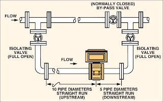
Figure 4: Horizontal installation of in-line meter

Technical texts courtesy of Omega.

Industrial Automation and Mechatronics

Labels

Announcement

Pages - Menu

Blog Archive

About